
Suppose you were presented with the following four graphical representations of datasets  with the question: which of the following data sets follow a linear model?
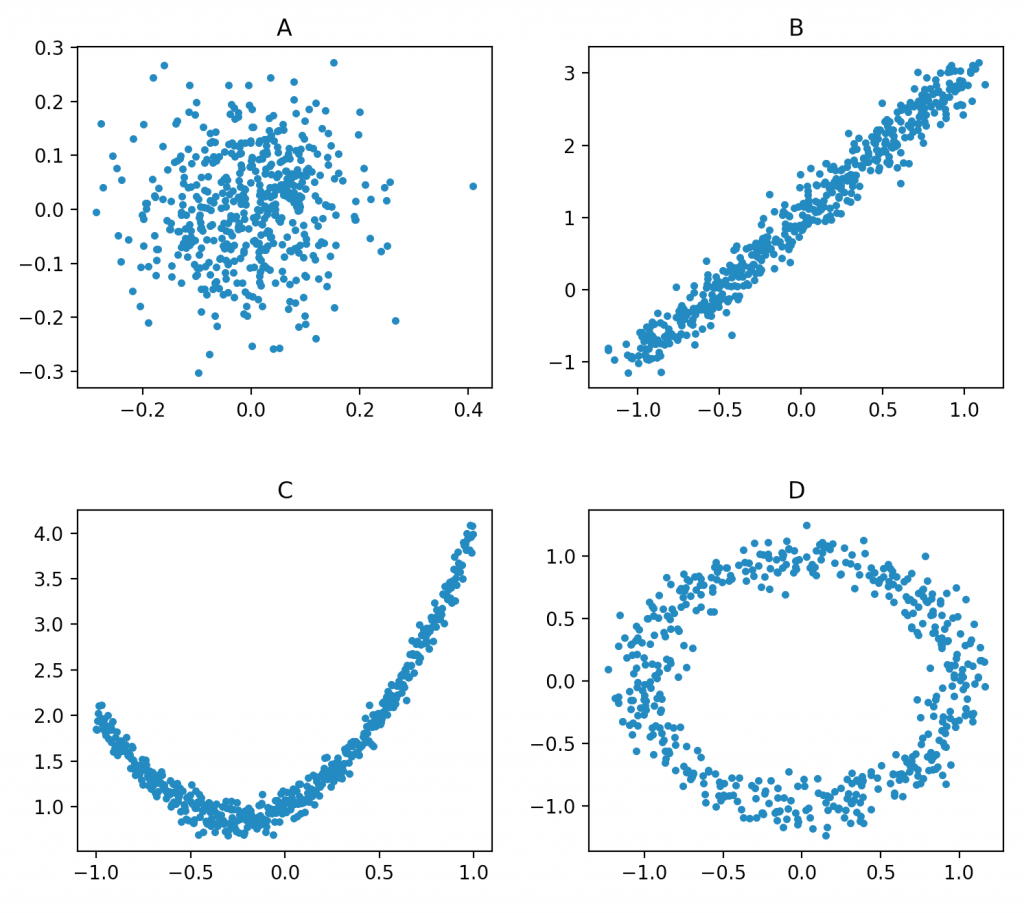
Almost everyone will agree that B is linear. Some might also add A to the list of linear models, and very few would say that C and D are linear. In this article I will show that A, B, and C are in fact linear models, with a caveat regarding C, and D is linearizable with the same caveat as C.
First we want to understand what it means to be linear. I find the most practical definition to be: if we can solve the model using least squares (a closed form solution) then we have a linear model. But in this definition lies a lot of interesting nuances. Let’s start with something classic, one dimensional linear regression (or what we have in dataset B).
Most of us are familiar with the representation:


![\mathbf{\beta}=[\beta_0, \beta_1]^T](https://www.riskideas.com/wp-content/ql-cache/quicklatex.com-491096d0b064912168d4bbea954e1b10_l3.png "Rendered by QuickLaTeX.com") ,
, ![\mathbf{y}=[y_0, ..., y_N]^T](https://www.riskideas.com/wp-content/ql-cache/quicklatex.com-81c8a6509e4dd8e2f647ea0082f0919c_l3.png "Rendered by QuickLaTeX.com") ,
, ![\mathbf{x}=[x_0, ..., x_N]^T](https://www.riskideas.com/wp-content/ql-cache/quicklatex.com-f25ef5f1bb58c78bcb8e63f37072c87e_l3.png "Rendered by QuickLaTeX.com") and
and ![X=[\mathbf{1}, \mathbf{x}]](https://www.riskideas.com/wp-content/ql-cache/quicklatex.com-342e91f462c5e9bf819870b43a449160_l3.png "Rendered by QuickLaTeX.com") . Unfortunately, simply memorizing formulas hides the magic that acts underneath. So let us unpack the least squares regression with a bit of derivation.
. Unfortunately, simply memorizing formulas hides the magic that acts underneath. So let us unpack the least squares regression with a bit of derivation.
The linear model above was somewhat misleading. Truly, the full representation pays attention to the error term:


Now suppose that  is normally distributed, then we have:


To get the best model we want to maximize the likelihood of the joint distribution over the parameter  . Instead of finding the maximum directly, we can also find the maximum of the log of the joint distribution, since both will share the same maximum point because the log function is one-to-one. Taking the log we see the negative sum of square errors, and negating the negative leads us to minimizing the square errors instead – giving us the least squares regression.
Considering this derivation, we can now give a more fundamental definition of a linear model:
A data generating process is linear if for any sufficiently large sample,  , there exist functions:
 that is parameterized by and linear in the variables
 that is non-constant over
 that is parameterized by and linear in the variables
 that is non-constant over
such that the sum of  and
and  describes an N-dimensional normal distribution over the data.
Let’s take this definition and see if we can apply it to cases A to D above.
Model A
If we define ![f((\mu_x, \mu_y)|(x_i, y_i))=[\mu_x, \mu_y]^T](https://www.riskideas.com/wp-content/ql-cache/quicklatex.com-700028a77f5a80568629f7c6fd780a68_l3.png "Rendered by QuickLaTeX.com") and
and ![g(x_i, y_i)=[-x_i, -y_i]^T](https://www.riskideas.com/wp-content/ql-cache/quicklatex.com-578321152bdda62e596dc12c8dbacdeb_l3.png "Rendered by QuickLaTeX.com") , then our function defines a 2-dimensional normal distribution,
, then our function defines a 2-dimensional normal distribution,  . The below code demonstrates this (including the code that was used to generate the data):
import numpy as np

rands = np.random.normal(size=1000)
x = rands[:500]/10
y = rands[500:]/10

Y = np.array([x, y])
Y = np.expand_dims(Y, -1)
X = np.ones(Y.shape)
beta = np.squeeze(np.matmul(np.matmul(np.linalg.inv(np.matmul(np.transpose(X, [0, 2, 1]), X)), np.transpose(X, [0, 2, 1])), Y))

print(beta)  # prints (will differ slightly per run): [-0.00205515 -0.00054436]
Before moving to Model B, let’s first analyze this result. Firstly,  turns out to be the average values of . Secondly, we use the data for the dependent variable and let the regressor be constant. This second point is very important, since the least squares regression won’t work otherwise. Thirdly (and finally), we did two independent linear regressions, and we can describe this process by a 2-dimensional linear model:
![$$[x_i, y_i]^T = [\mu_x, \mu_y]^T + N(0, \Sigma)$$](https://www.riskideas.com/wp-content/ql-cache/quicklatex.com-73af72824b60725ad5238f7feeb7de88_l3.png "Rendered by QuickLaTeX.com")
 is a normal distribution generator.
Model B
We did this one already, but let’s add it here for completeness. If we define  and
and  , then our function defines a 1-dimensional normal distribution. And the code:
import numpy as np

rands = np.random.normal(size=1000)
x = np.arange(-1, 1, 0.01/5*2) + rands[:500]/10
y = 2*x+1 + rands[500:]/10

Y = y
X = np.expand_dims(x, -1)
X = np.concatenate([np.ones(X.shape), X], -1)
beta = np.squeeze(np.matmul(np.matmul(np.linalg.inv(np.matmul(np.transpose(X, [1, 0]), X)), np.transpose(X, [1, 0])), Y))

print(beta)  # prints (will differ slightly per run): [0.99938605 1.94454423]
And the results are as expected. We’ll move on to the next model since there is not much new to see here.
Model C
For this one, let’s try some polynomial. If we define  and , then we are also 1-dimensional. The code:
import numpy as np

rands = np.random.normal(size=1000)
x = np.arange(-1, 1, 0.01/5*2)
y = x+1+2*x**2 + rands[500:]/10

Y = y
X = np.expand_dims(x, -1)
X = np.concatenate([np.ones(X.shape), X, X**2, X**3, X**4], -1)
beta = np.squeeze(np.matmul(np.matmul(np.linalg.inv(np.matmul(np.transpose(X, [1, 0]), X)), np.transpose(X, [1, 0])), Y))

print(beta)  # prints (will differ slightly per run): [0.97756608  1.01012193  2.10034334 -0.0032706  -0.10355826]
Here we do have some new elements to analyze, so let’s take a moment. Firstly, notice that we did not add an element of randomness to the regressor,  . This is especially important to the linearity aspect. When both our dependent variable and regressors were linear in the data, then any randomness attached to their value was linearly added, still resulting in a normally distributed error term. However, squaring and so forth random normal errors does not result in a random normal error – try this out! Secondly, we would have been fine just fitting a second order polynomial, but even still our result showed us significant results only in the first three coefficients.
Model D
Some data that looks nonlinear is secretly hiding inside it a linear model. Cyclic time-series are one such example. Here, we don’t have a time-series, per se, but the data does exhibit some cyclicality in it. A suitable function can look like  and
and  . And the code:
import numpy as np

rands = np.random.normal(size=1000)
t = np.arange(-1, 1, 0.01/5*2)
x = np.cos((t + rands[:500]/10)*3.1459)*(1 + rands[500:]/10)
y = np.sin((t + rands[:500]/10)*3.1459)*(1 + rands[500:]/10)

r = np.sqrt(x**2 + y**2)
tt = np.arctan(y/x)

Y = r
X = np.expand_dims(tt, -1)
X = np.concatenate([np.ones(X.shape), X], -1)
beta = np.squeeze(np.matmul(np.matmul(np.linalg.inv(np.matmul(np.transpose(X, [1, 0]), X)), np.transpose(X, [1, 0])), Y))

print(beta)  # prints (will differ slightly per run): [0.99578537 -0.0028933]
We have much more to say here. Firstly, we see that our data fits a circle quite perfectly, as we could have done away with the  altogether – the resulting coefficient is insignificant. Meaning, we essentially have Model A but in a different space. Secondly, notice that unlike Model A, we started here with two input variables and ended up with only one average. We can say that we lost some information, but that is not entirely true. If we attempted to fit the data from Model A using this model, we would get some really bad results – again, I recommend trying it out. What we gained here is the relationship between the two inputs, that their square sum is 1. Try as you may to get better results and you won’t. Simply put, we were able to reproduce the underlying generating model perfectly, so any more and we will simply be wrong!
In this last section I want to dedicate a few lines to bring all these examples together and circle back to the definition we gave for a linear model above. Firstly, we may ask what good is building models on transformations of the original data, because what interests us is the data, not some other derived data – i.e. we want some  . So two things:
- The representation above is excellent for anomaly detection, and this is actually how all statistical anomaly detection methods work – detect some underlying pattern to the data, both
 and
and  , and see if they lie within the pattern. The framework above works with this pattern perfectly.
 - If we merely aim for
 then we precondition to be the dependent variable and to be the regressor, when it could be the other way around or neither at all. In fact, this framework for thinking about regression will always fail to explain something like Models A and D.
 and
and  , and see if they lie within the pattern. The framework above works with this pattern perfectly.
If we choose to go with the  approach above, then we are able to model a larger class of relationships – even going as far as the behavior in Model D. Furthermore, we have a closed-form technique to solve for the model, which greatly saves compute time (and degrees of freedom) in implementing gradient descent on non-linear sections of a potentially more complicated model.
However, we need to be careful in how we think of “linearizing” models. An important criteria is that  must be normally distributed over the data, while
  is linear in the parameters and
  is non-constant over the data. This is not always the case, and we must pay attention to (and test) this hypothesis before accepting the results.